Page Contents
Page 2
Change particles based on distance to a point
This is another easy one. We will use the pCustom tool to calculate the distance of each particle to a specified point. This will be the first time in this tutorial series where we will use the Point inputs of this tool. You can create some really cool motion graphics effects with this method.

We only need a pEmitter, the pCustom, and of course the pRender.
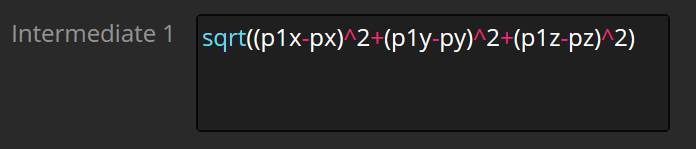
In the Intermediate-Tab of the pCustom:
sqrt((p1x-px)^2+(p1y-py)^2+(p1z-pz)^2)
This is essentially all we need as this will calculate the distance each particle (px, py, pz) has to the Position 1 point (p1x, p1y, p1z) in the Positions-Tab.
Try this, go into the Particle-Tab and put “i1” into the Red, Green and, Blue-fields. Give your particles some velocity (or spawn them in a big area) and you will see them being black and the center and brighter the further they go away from the point.
When you move the point, the values will change accordingly.
But this is barely art direct-able. For example, if we want to change the size of these particles based on distance. they would simply get bigger and bigger. This is why we need to remap these values. The first result on Google shows you what we need to do to remap values.
We need to know our previous lower limit (always 0) and our previous upper limit, which is always increasing. This is why we will first clamp these values.
In the Intermediate-Tab of the pCustom:
Intermediate 1: clamp(sqrt((p1x-px)^2+(p1y-py)^2+(p1z-pz)^2), 0, n3)

I have highlighted what is new. It’s the clamp() function. As the name suggests, it simply takes a value (currently the distance from Point 1) and stops it from going below or above the specified values. We will use the Number 3 (n3) input for that. This will later work as a falloff control.
Next, we need to do the actual remapping of values. We will use the algorithm linked above, but since our old minimum is always 0, we can get rid of some of the characters.
In the Intermediate-Tab of the pCustom:
Intermediate 2:(((i1) * (n2 - n1)) / (n3)) + n1
In the Particle-Tab change the Red, Green and, Blue-fields from “i1” to “i2” and dial in the values in the Numbers-Tab.
As you can see, now you have control over the falloff (n3), the minimum value (n1), and the maximum value (n2).
Play around with this. You can do a lot with this, not only change colors. Another obvious way would be to control the size or position (think of Cinema4D’s mograph toolset with fields). Or write it into the user attribute to carry it to a pCustomForce.
Download this Example here:
DownloadPlace Particles on a mesh surface
You can spawn particles on a mesh already using the standard pEmitter tool, but that’s always more or less random. With this setup here, you can create some awesome particle meshes that can be combined with other particle forces for incredible effects. To create some holographic looking effects for example.

As you can see in the image above, we are going to use a pImageEmitter this time. This does also work using the standard pEmitter but that’s harder to get right. (And it has no advantages to the pImageEmitter.)
We also need a Shape3D, a ChannelBoolean3D, and a Render3D tool. This is because we are going to render the current world position of each vertex to use this as our particle starting position.

Pipe the ChannelBoolean3D into the material input of the Shape3D and in the ChannelBoolean3D set Red, Green, and Blue to their matching position. As seen in the image.
Also change it to work in World space instead of Object space.
If you are using the Cube as your shape, remember to set it to Cube Mapping in the Shape3D settings to get proper UV islands for all six sides.
Next, pipe this into the Renderer3D and set the render Type to OpenGL UV Renderer. As the name suggests, we are not rendering a scene by looking through a camera but rather UV unwrap the Shape which currently tells us the position each vertex has.
This also means, you need to have UV’s on meshes you import from somewhere else. Or this will not work. For example, the Runner I am using throughout the videos, shares the same UV island for both shoes. That is why there are particles being placed only on one of the shoes.
Remember to set the output resolution of this Render3D to something with one by one aspect ratio like 64×64.

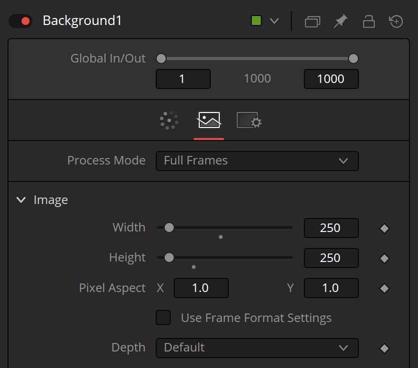
Now, we could pipe this image into the pImageEmitter or use a different image. I have chosen a simple white Background tool. This has to be the same resolution as the Renderer3D. You also want to keep your resolution fairly low as this will already generate a ton of particles.
Next, we will make the magic happen inside the pCustom tool. We only need to change the positions of each particle. We do that by referencing the image of the Render3D tool, which renders out the position of our Shape3D.
So pipe the output of the Render3D into the the Image 1 input of the pCustom tool.
You also want to change the duration of when this pCustom tool is active to only the first frame of a particles life.
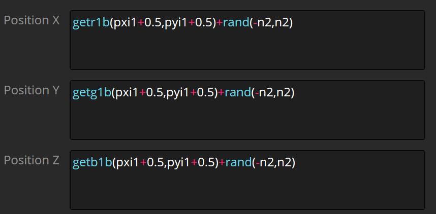
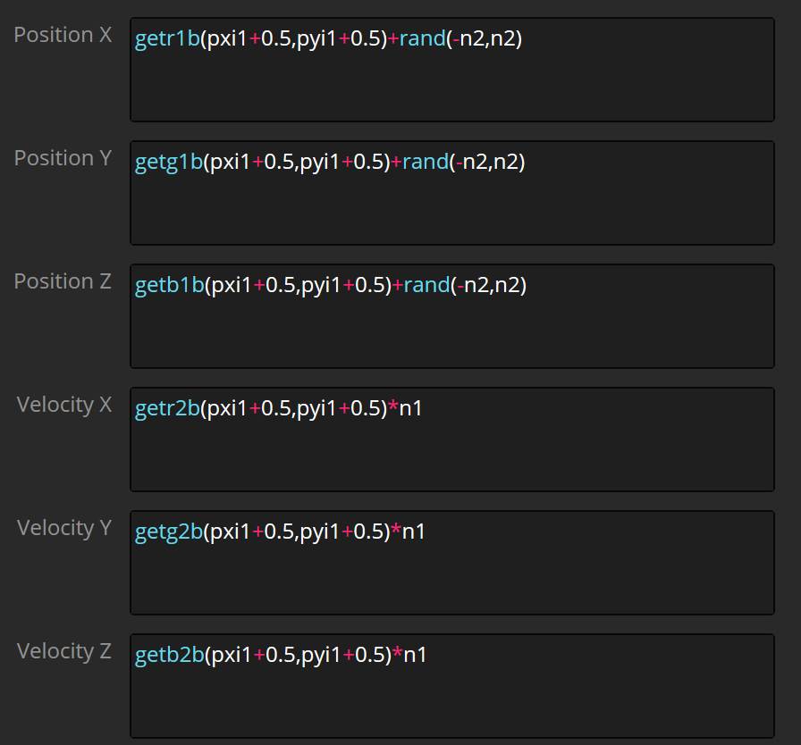
In the Particles-Tab:
Position X: getr1b(pxi1+0.5,pyi1+0.5)+rand(-n2,n2)
Position Y: getg1b(pxi1+0.5,pyi1+0.5)+rand(-n2,n2)
Position Z: getb1b(pxi1+0.5,pyi1+0.5)+rand(-n2,n2)
What is going on here?
We use getr1b(X, Y) to get the information of the red channel of the first image input. Remember this works on each particle individually and we need to tell the getr1b(X,Y) function which pixel it should get the information from. This is why we use pxi1, as this is the current particle position converted to a 2D plane and corrected for the image 1 aspect ratio. The same applies to pyi1.
We also need to correct this to the origin, this is why we add 0.5 to both the X and Y position.
getr1b(pxi1+0.5,pyi1+0.5)+rand(-n2,n2)
I also added another (optional) random function, to vary the position.
And that is all to position them on a surface mesh. But you know what would be cool? If they would inherit the velocity of the mesh as well. And that’s exactly what we will do in the next example.
Download this Example here:
DownloadParticles inherit mesh velocity
By default, when using a 3D mesh to emit particles, you can’t make the particles inherit the velocity of the mesh. This actually has been an issue for me several times in the past when doing VFX work that includes magical effects.
But we can use the previous setup and add some functionality to it, to achieve exactly that.
This isn’t something I came up with myself though. I found this method in the WSL Forum, unfortunately, I can’t seem to find that post again. If I do, I will link to it.

But the idea is simple, we use the exact same setup as before to place the particles on the mesh. But this time we will calculate the speed of the mesh and set that to the Velocity-fields in the pCustom tool.
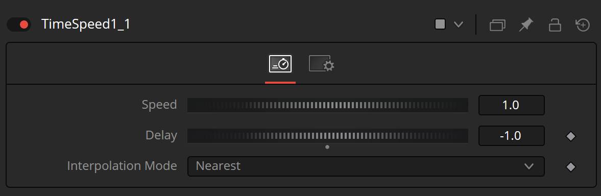
Calculating the velocity is simple. We need two positions and subtract their values. (I can’t believe my teachers were right. I do use math in my life). We achieve that by using a TimeSpeed tool. Keep the Speed at 1 but change the Delay to -1 and the Interpolation Mode to Nearest (just to be safe).
Plug the Output of the Render3D into the TimeSpeed tool and place down a ChannelBoolean tool. The Timespeed should be plugged into the Background Input and the Output of the Render3D into the Foreground Input of the ChannelBoolean.
Set the Operation to Subtract and pipe the Oupout of the ChannelBoolean into the second image Input of the pCustom tool.

In the Particles-Tab:
Velocity X: getr2b(pxi1+0.5,pyi1+0.5)*n1
Velocity Y: getg2b(pxi1+0.5,pyi1+0.5)*n1
Velocity Z: getb2b(pxi1+0.5,pyi1+0.5)*n1
What is going on here?
We are using the exact same method as before. We are reading the data saved into an image and apply it to the particles. Only this time we are using:
getr2b(X,Y)
This is because we need to read the data from the second image input, not the first.
And this second image contains the velocity or direction vector in its R, G and B channels.
We only multiply it by the number in n1 to have some control over the strength of the velocity. And of course, you could add a rand() function to it to add some randomization.
And that’s all for a pretty awesome effect.
In this example, we have created a direction vector to drive the initial particle velocity. In the next example, we will use motion vectors generated from videos to influence them.
So be sure to check out the next page.
Download this Example here:
Download

